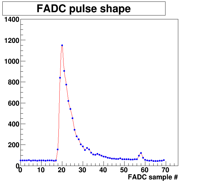
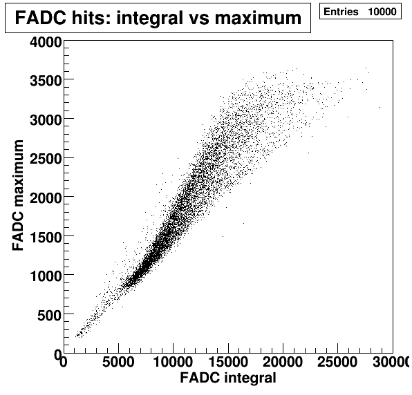
Notes on cosmic test of modules

1) FADC signal shape

Fig.1. Typical FADC signal shape Fig.2. Integral of FADC hit vs its maximum

Typical FADC shape is shown in Fig.1. Note the reflection 160ns after the signal.

a) Attempts were made to fit the "two and a half" points in the leading edge to determine time-walk corrections straight from the signal shape. This kind of works but not as good as a method shown below. However, I'm looking again at this approach after realizing that the highest sample may belong to the trailing edge rather than the leading one.

b) Fig.2 shows FADC hit integral (with pedestal subtraction) vs its maximum. I'm trying to determine what should I use for time-walk corrections (TWC) , and I don't see much difference. For small signals (where TWC are important), the dependence is almost linear.

2) High-voltage (gain) balancing

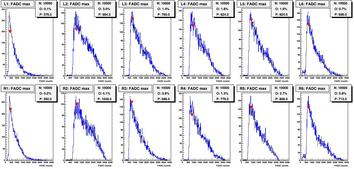
Fig.3. FADC maxima for 12 PMTs at 1500 V

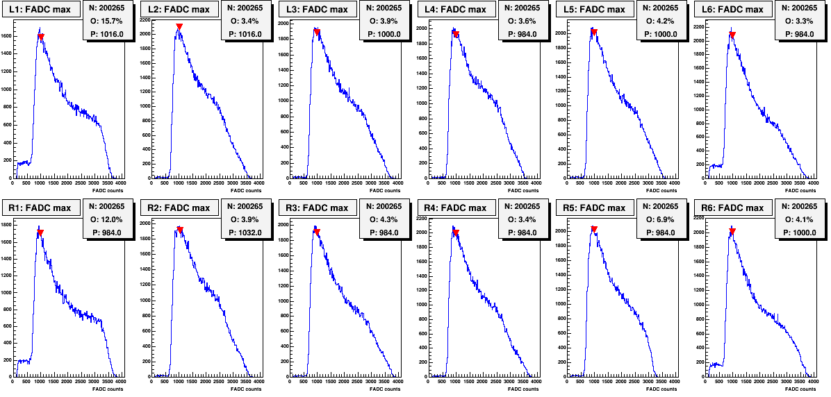
Fig.4. FADC maxima for 12 PMTs at their balanced HV

Distribution of FADC maxima over all hits for 6 bars (12 PMTs) is shown in Fig.3 for all PMTs at initial HV of 1500 V, and in Fig.4 after HV balancing is done. Value "P" in the stats box denotes the position of the most probable hit. The goal is for the most probable value to be at 1000 counts (+-5%). This roughly corresponds to 500mV signals.

The improvement to the algorithm was made. It was determined that the peak position follows the dependence of P=exp(a+b*HV). So, instead of just trying with 25V steps, the next HV setting is determined from the exponential fit of the previous 2 measurements (starting initially with 1500 V and 1750 V). This allowed to cut down from 6-7 tries to 4 or 5 attempts.

Fig.5 shows the correlations between balanced HV and nominal PMT gain for 24 PMTs (12 modules) tested so far. They mostly follow a certain dependence which indicates that there is no unusual light loss due to glued joints or "forgotten" ESR protective film. Only a bar with 2 lowest-gain PMTs seems to be off the track. However, we need to test a few more low-gain modules for comparison. At the moment, this bar is not a suspect yet but just "a module of interest". Note also, the amount of very large pulses (overflows "O" in the stats box of Fig.4 of L1&R1) is much higher for this particular module. We may revisit this module later.
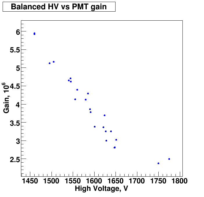
Fig.5. Balanced HV value vs nominal PMT gain


3) Time-walk corrections

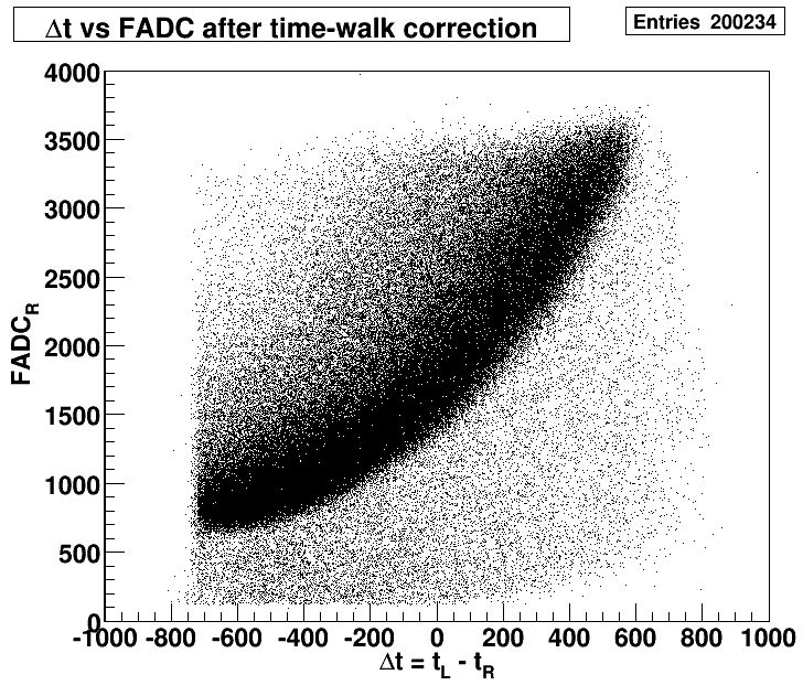
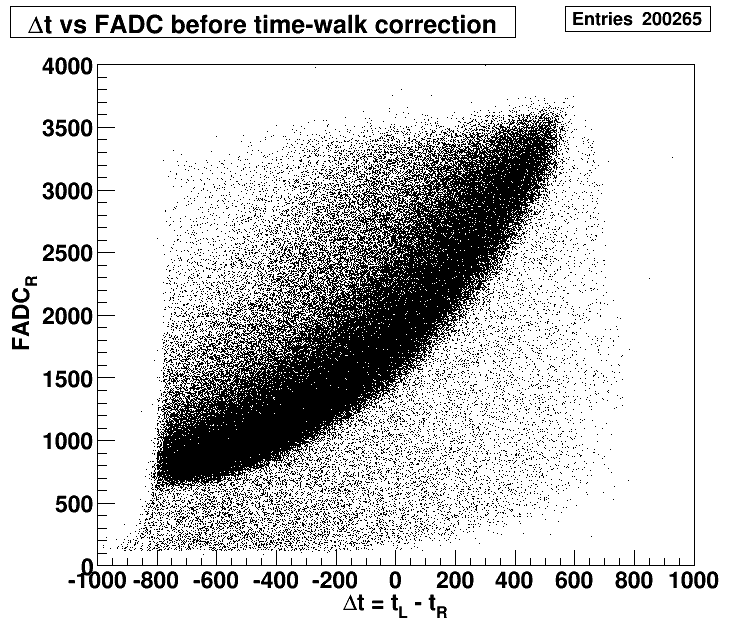
Fig.6. Time difference vs FADC max before and after TWC

As a measure of time-walks, I look at the lower-left corner of Delta(t) vs FADC max distribution shown in Fig.6. A simple form t_cor = t - b/sqrt(FADC) is used for TWC. The fit tries to minimize the skewness of this distribution (and the similar one for PMT at the other end), and it seems to succeed at that.

The corrected figure is also used for two other purposes: a) to determine the speed of light, assuming that the width of the distribution corresponds to 254cm paddle length; b) Exponential fit of the band gives light-attenuation length.


4) Possible data selection cut

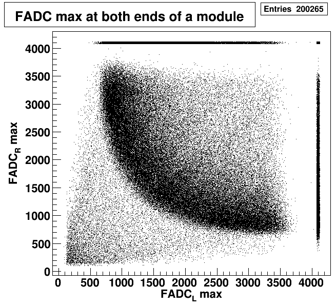
Fig.7. FADC left vs right

Fig.7 shows a clear band for minimum-ionizing particle. The smaller hits may be from scratching the edges. Or even from triggering on reflection rather than the main signal. Some very large signals may originate from the photocathode HV discharge. I'm implementing "a banana cut" of MIP band for the purpose of time resolution determination.

5) Mystery of trigger timing jump

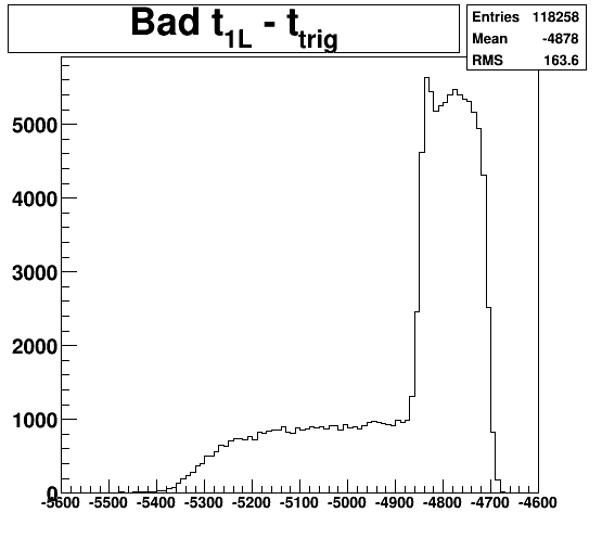
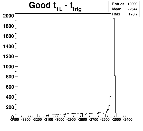
Fig.8. Time difference between L1 (left bottom) PMT and trigger

The trigger is set as a logical AND of 12 PMT signals. The signals intially go into 50/50 passive splitters. One output goes into FADC, the other one goes into JLAB LED. Discriminator has 2 sets of ECL outputs: one goes into CAEN TDC, the other one - into ECL-NIM level converter. From there, the signals are sent through the chain of NIM 4-fold coincidence units to form the final trigger for TDC and FADC stops. Trigger also goes into TDC as a normal input to measure its timing. The trigger time is basically the time of the latest among all 12 hits plus some fixed additional time to form the trigger in the NIM logic.

Well, mysteriously, this fixed time became not so fixed at some point. During the whole test of batch #1 and initially for batch #2, the TDC time difference between a signal from one of 12 PMTs and a trigger looked like Fig.8(left). The shape consists of two parts. When a hit is in the module's half which is closer to the side of this PMT, its the other side which determines the trigger time. Therefore, time difference with a trigger looks similar to the time difference with the opposite PMT. I.e., it looks like a normal Delta(t) distribution. However, when a hit is in the module's half away from the PMT, trigger time is determined by the same side as the PMT, and time difference becomes delta-function. The width of this peak is due to electronics resolution and due to different incident angles (under large angles, its the top paddle rather than the bottom one which has the latest signals). So, the general shape of the distribution is as expected.

However, sometime in the middle of batch #2 measurements (and without any changes to anything), the trigger time got an additional ~55ns delay as seen in the shift from left to right figure. Also, a delta-function got 2-3ns width due to some unknown jitter.

Checking signals with the scope didn't reveal anything. 2-3ns jitter cannot be seen when relative timings change upto 17ns from event to event due to hit position. Also, half of the signals are in ECL which is not trivial to see. Relative (to each other) timing of the incoming PMT signals didn't change. So, I'm still trying to find the cause of the mysterious 55ns jump and 3ns jitter...